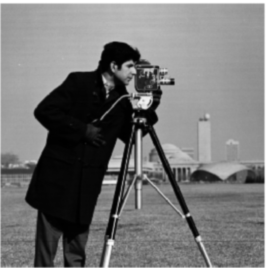
Part 1.1: Finite Difference Operator
\[
\mathbf{D_x} = \begin{bmatrix} -1 & 1 \end{bmatrix}, \quad \mathbf{D_y} = \begin{bmatrix} 1 \\ -1 \end{bmatrix}, \quad
\| \nabla f \| = \sqrt{\left( \frac{\partial f}{\partial x} \right)^2 + \left( \frac{\partial f}{\partial y} \right)^2}
\]
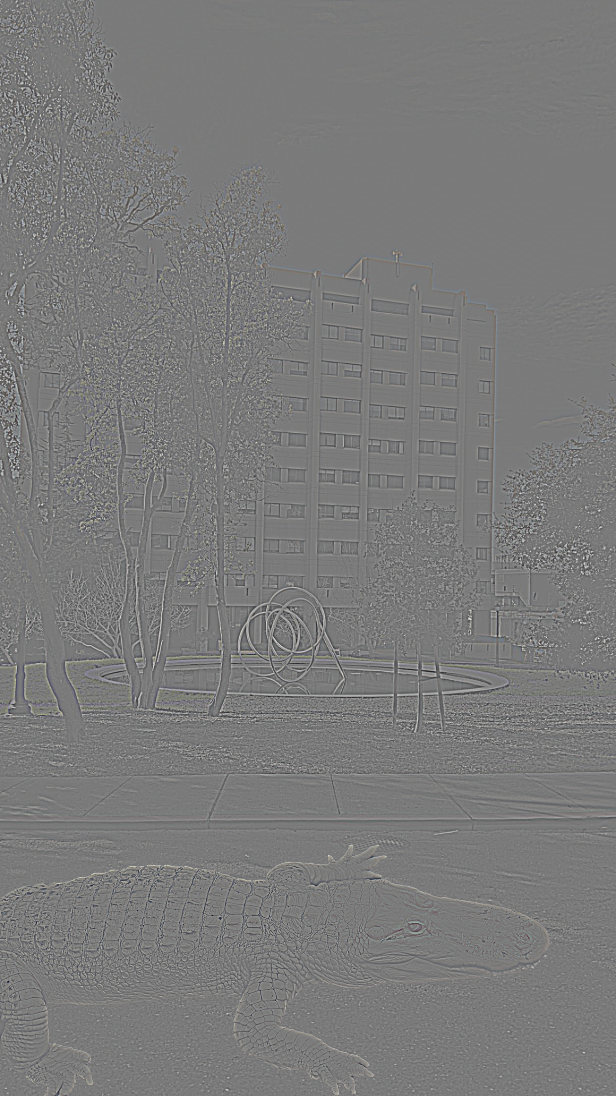
By convolving the image with a difference operator, we can create a map to see the change in spatial frequency. In other words,
we are seeing the change in the intensity of the pixels' brightness as we move across the image.
For example, areas where this change in spatial frequency is high is on the edges of an image. So, we can use this idea to edge detect.
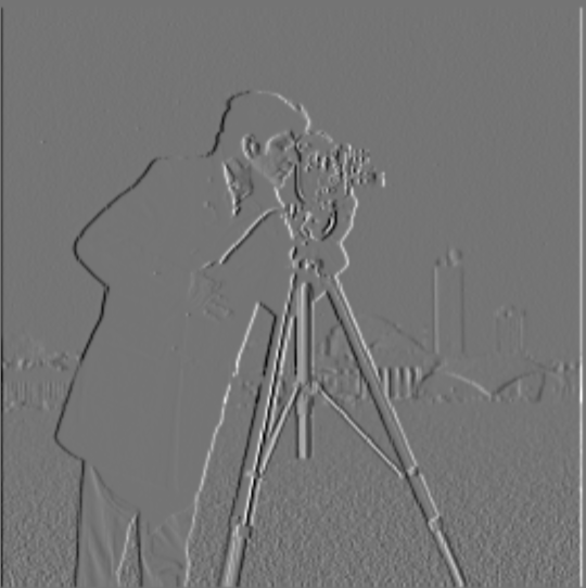
The approach is to take an image and convolve it with the finite difference operator in each direction, x and y, then calculate the
magnitude of the gradient which will give the total rate of change in intensity, regardless of direction. We then binarize the image
by choosing a threshold to remove as much noise as possible whilst perserving most of the real edges. To binarize the image,
pixels that are greater then some threshold get set
to 1; otherwise, they are set to 0. Playing around with the threshold number
allows us to remove the noise.
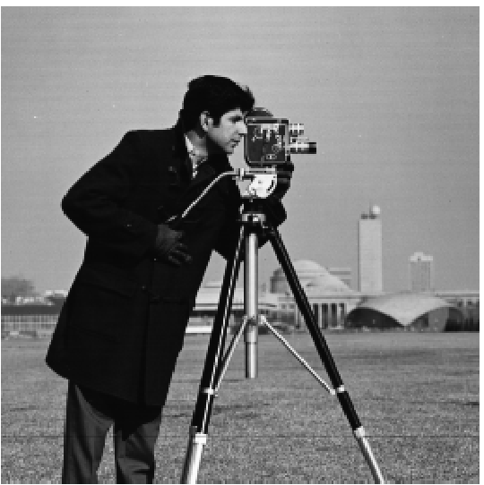
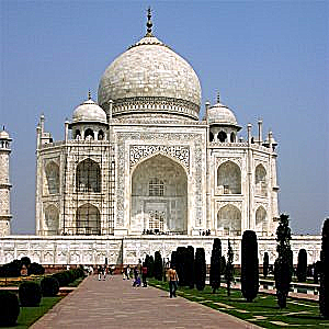
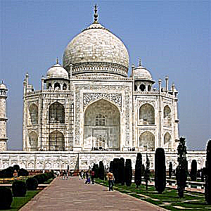
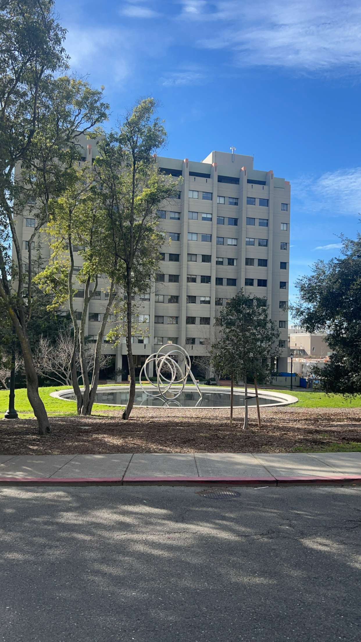
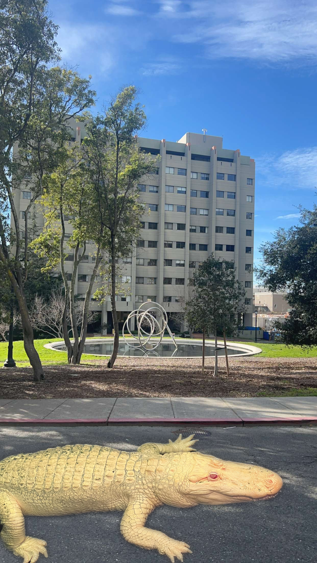
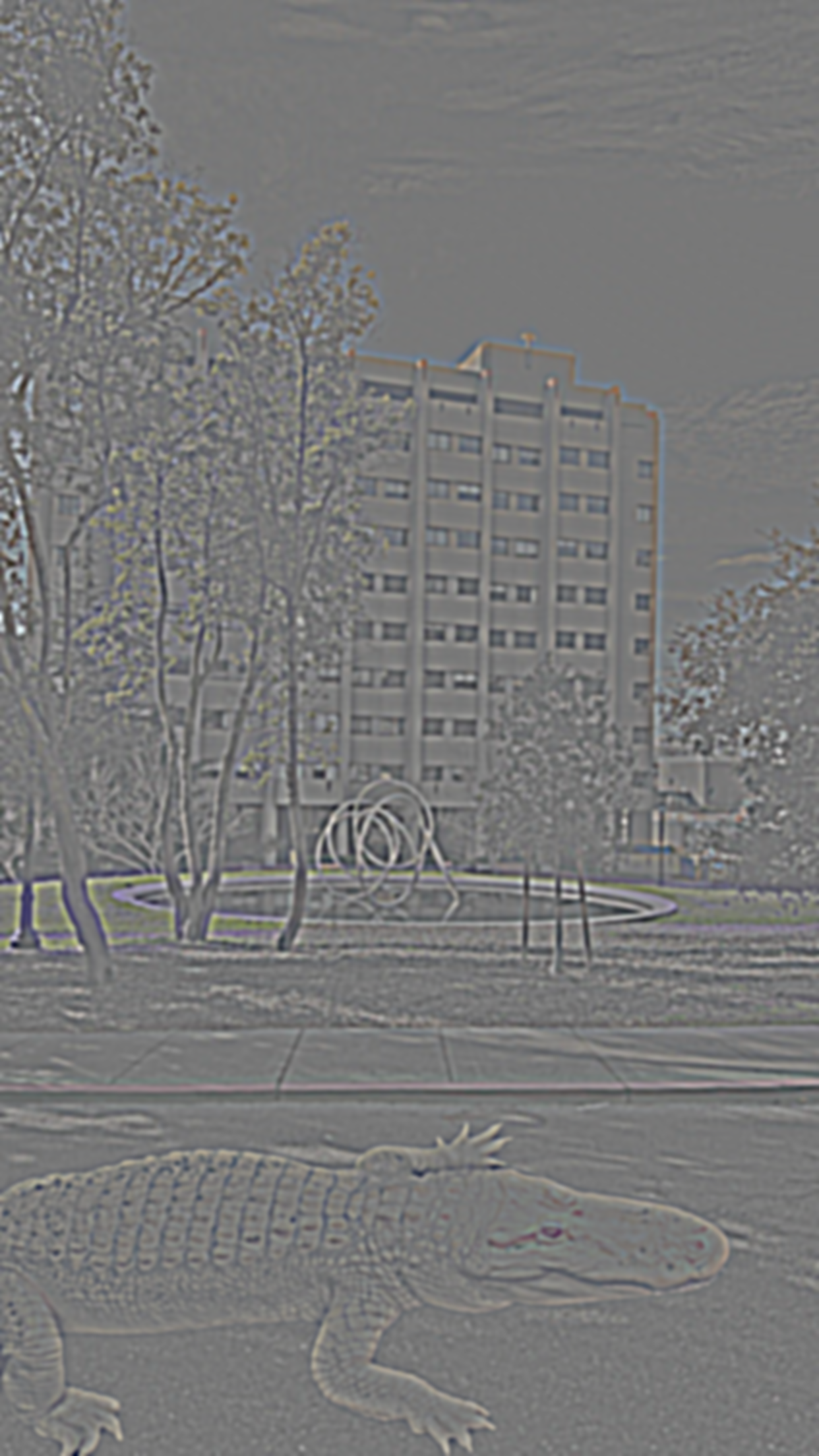
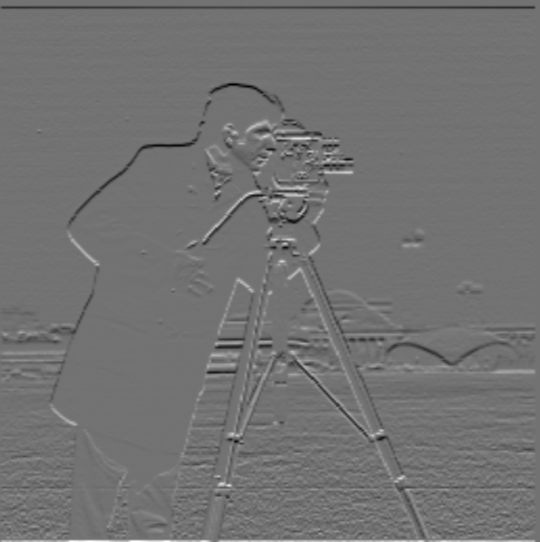
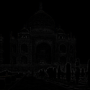
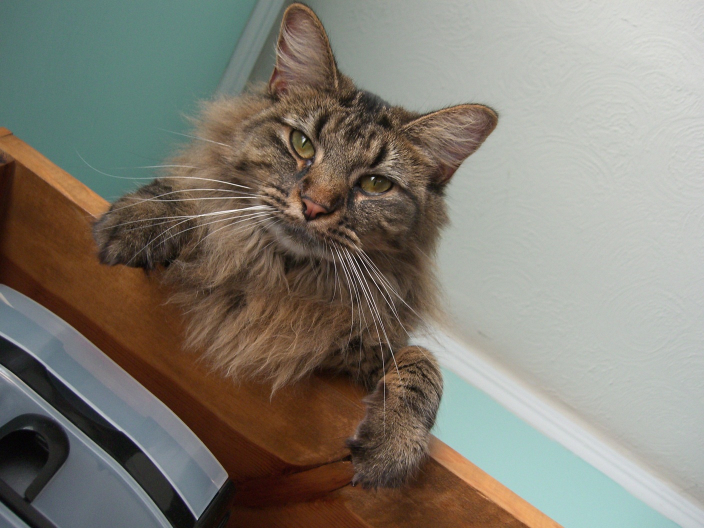
Original
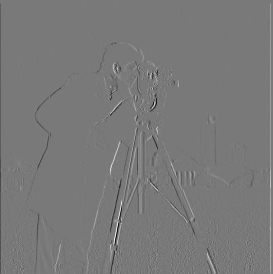
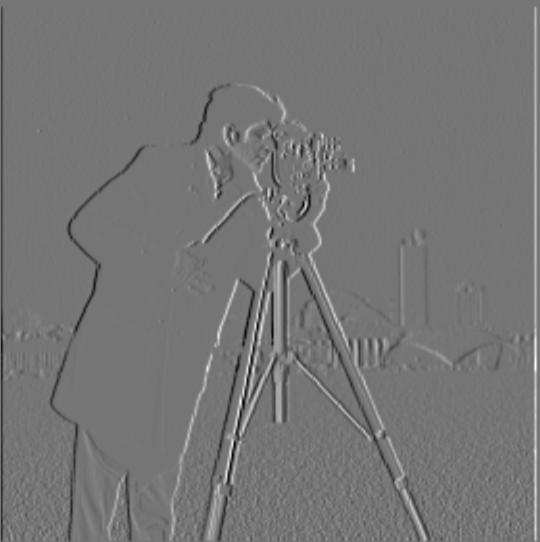
Partial derivative in x-direction

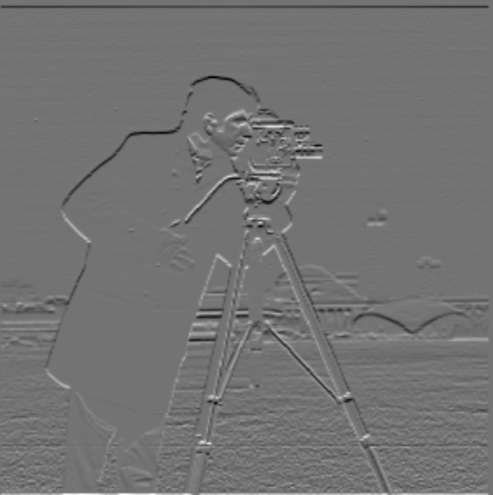
Partial derivative in y-direction
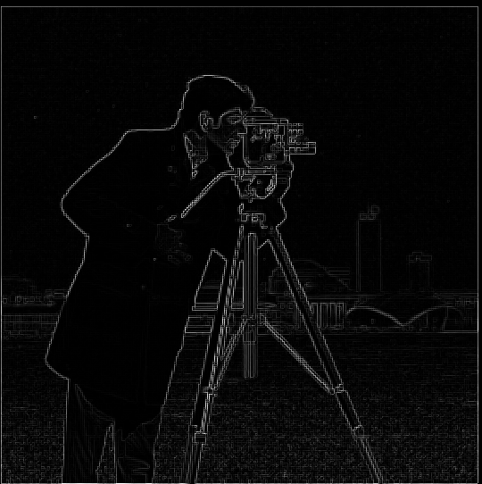
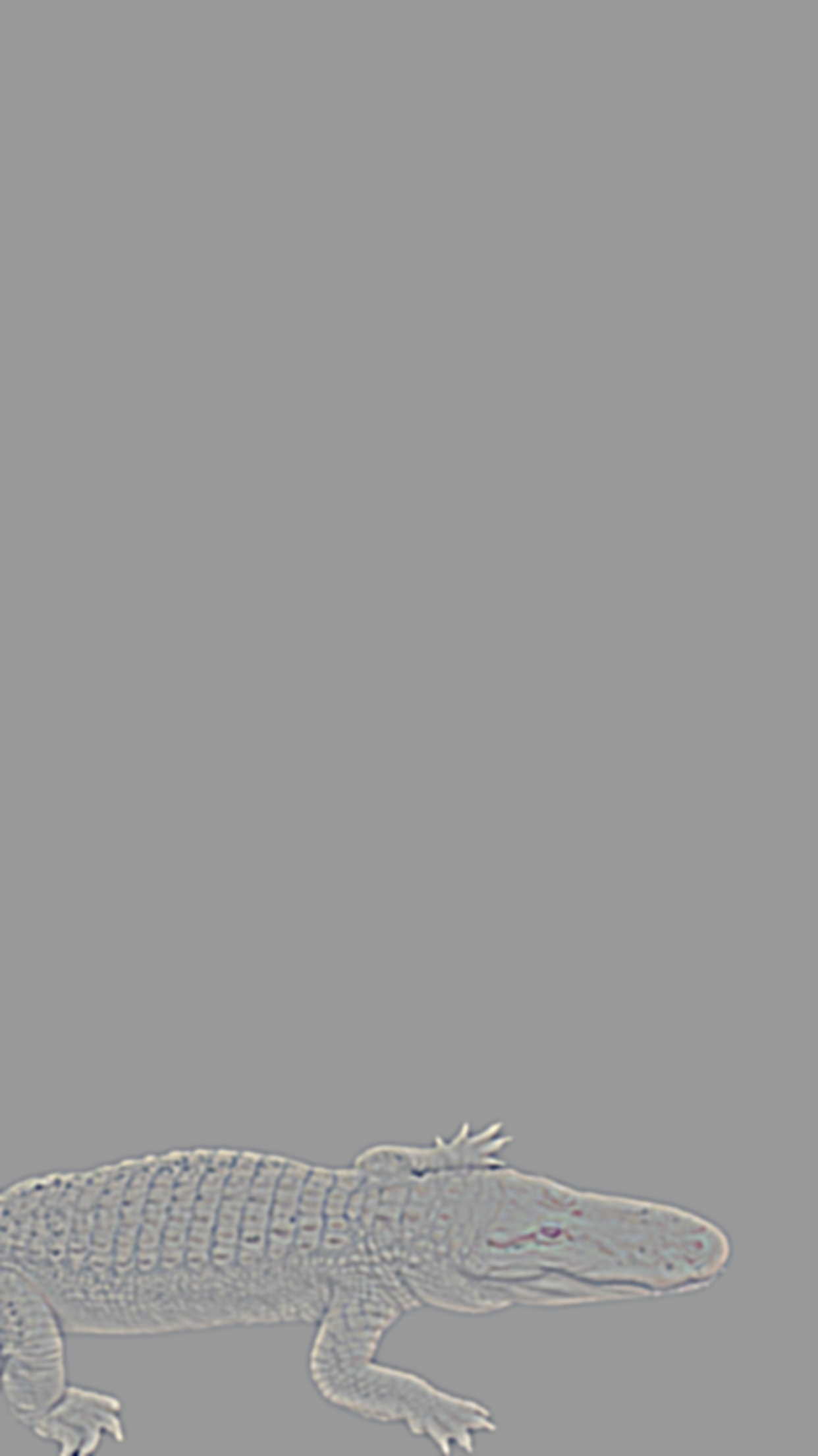
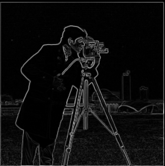
Gradient Magnitude
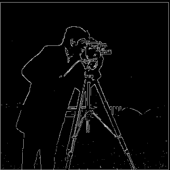
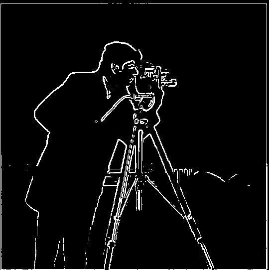
Binarized (Threshold = 67)
Part 1.2: Derivative of Gaussian (DoG) Filter
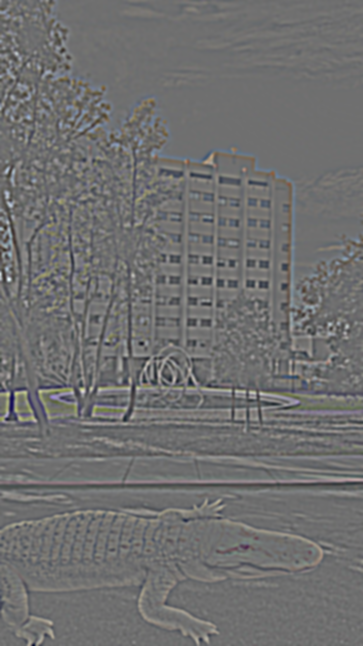
As seen in the partial derivative images, it is quite noisy, especially near the grassy area. This throws off our edge detection, as seen in the binarized
image.
We can remedy this by blurring the image first, and then applying a difference operator. The smoothing/blurring acts as a low-pass filter -
smoothening out the higher frequencies, since the edges have very high frequency they will still be relatively preversed in the filtered image.
1. Applying Gaussian blur then applying finite difference operator in each direction.
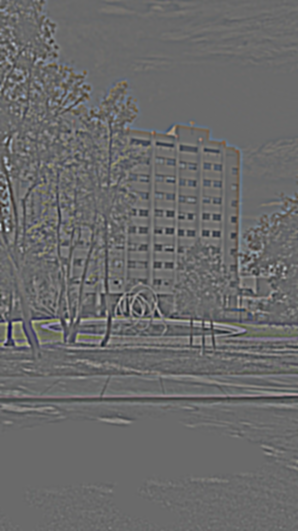
Gaussian Blur (σ = 1)
Partial derivative in x-direction
Partial derivative in y-direction

Gradient Magnitude

Binarized (Threshold = 28)
Reflection: After smoothening the image, the edges have become more distinct. The noise has also
decreased.
2. Convolution is commutative and associative, so it is possible to take the difference of Gaussian.
In other words, we can convolve the difference operator and Gaussian kernel to create a DoG filter,
and then apply it to the image.
Partial derivative in x-direction
Partial derivative in y-direction
Gradient Magnitude
Binarized (Threshold = 28)
Reflection: As suspected the result is the same.
Part 2: Fun with Frequencies
Part 2.1: Image "Sharpening"
We are able to sharpen images by adding some of the higher frequencies back to the image. This is achieved by doing a low-pass filter on the original image
then subtracting it from original image. This leaves us with an image with high frequencies that we can add back to the original image. We can also multiply the
high frequency image by a scaler (alpha) to sharpen the image further.
Original

Low Frequencies
High Frequencies

Original
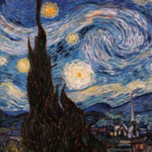
Low Frequencies
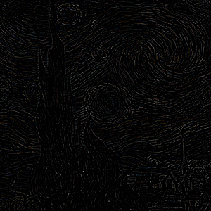
High Frequencies
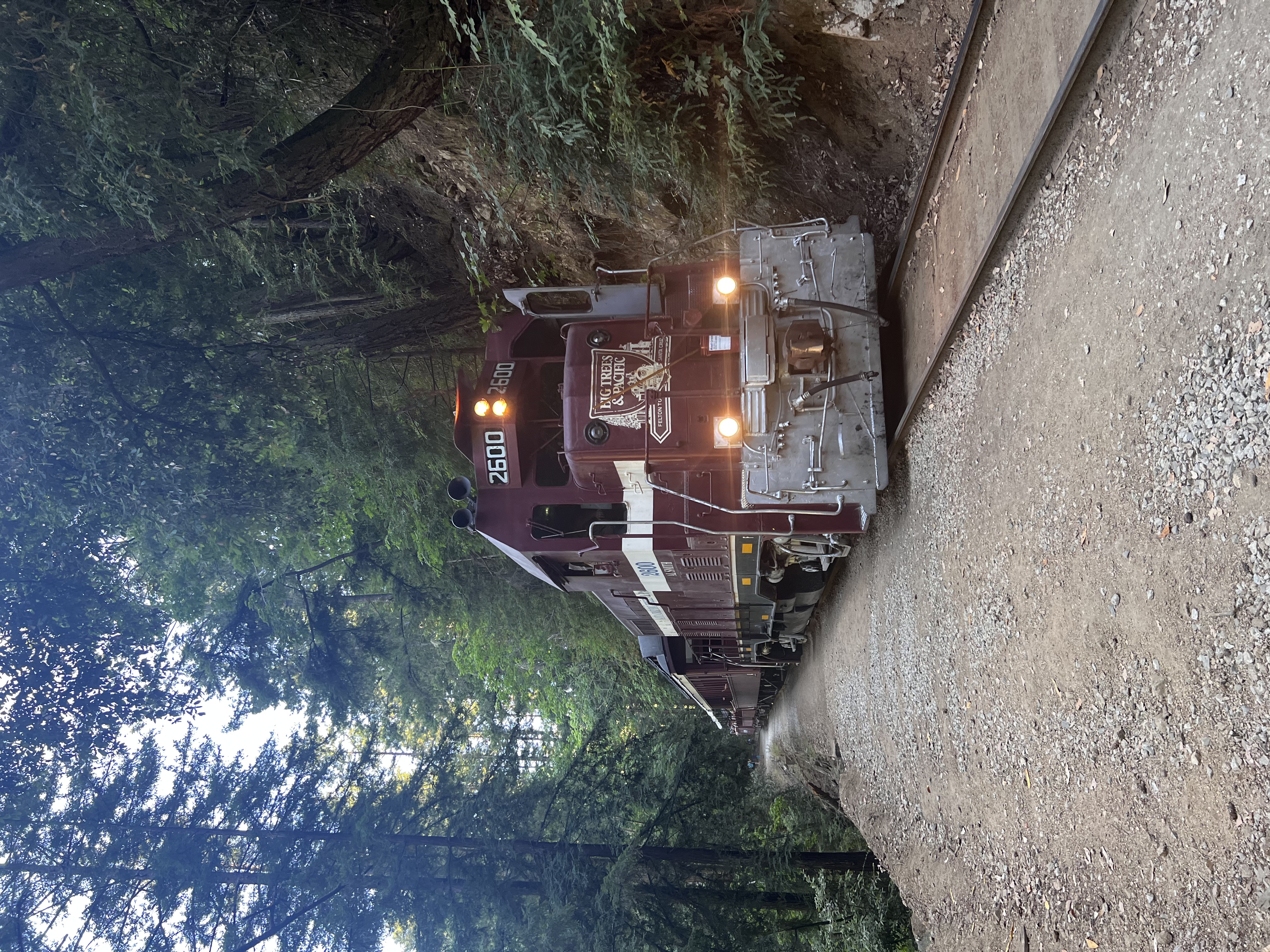
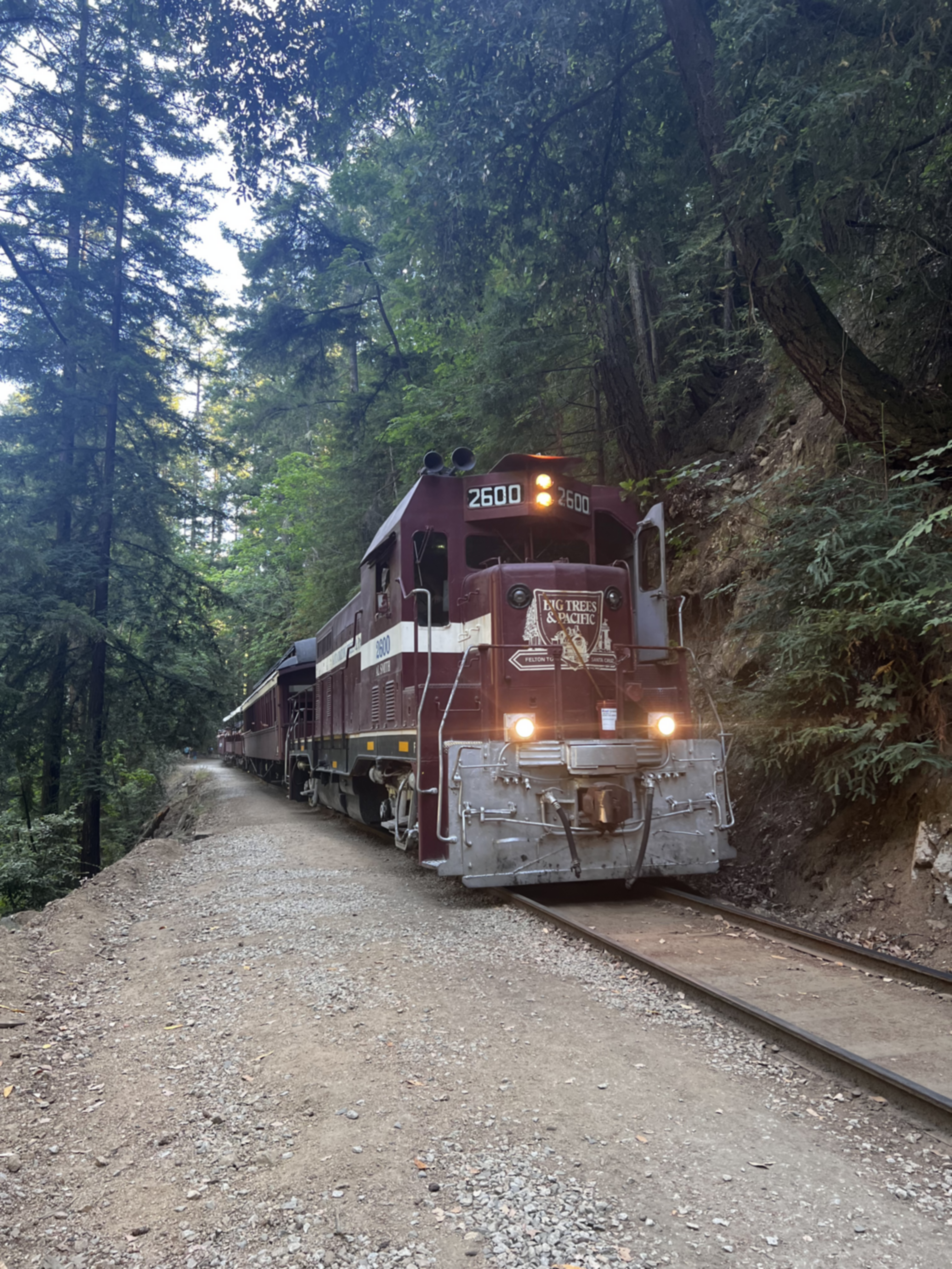
A picture of a train from my phone's camera was already sharp. After blurring it, and sharpening that blurred image, the image didn't see any drastic change. This may have been because of a low alpha or low sigma. I tried to see if that
was the case, but it took too long to run on my computer, so I wasn't able to test it.
If you look closely, some of the writing on the train got sharper, but it is very subtle. The original image still looks better because sharpening
can't restore the loss of detail from the blurring.
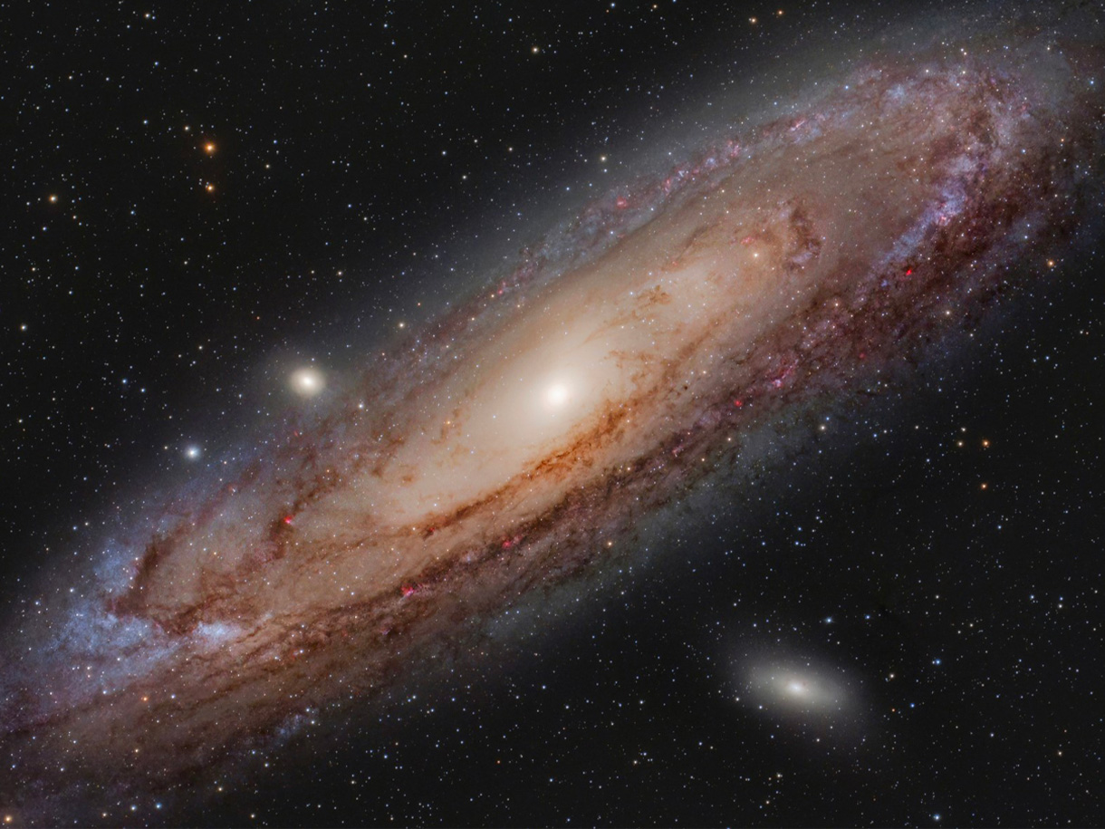
Part 2.2: Hybrid Images
We can create images that look different up close and farther away; they are called hybrid images. This is done by keeping the higher frequencies of one image
and the lower frequencies of another. The higher frequency image is seen up close and the lower frequency image is seen from farther away.
I followed the approach outlined in a paper called Hybrid Images by Oliva, Torrabla, and Schyns.
The approach was to low-pass filter the image you want to be seen farther away and high-pass filter the other, and then add the images. The low-pass filter was a standard
Gaussian blur, and the high-pass filter was subtracting the Gaussian-filtered image from the original image.
I tried averaging the images, instead of adding, but I liked the look of the addition, so I stuck with that.
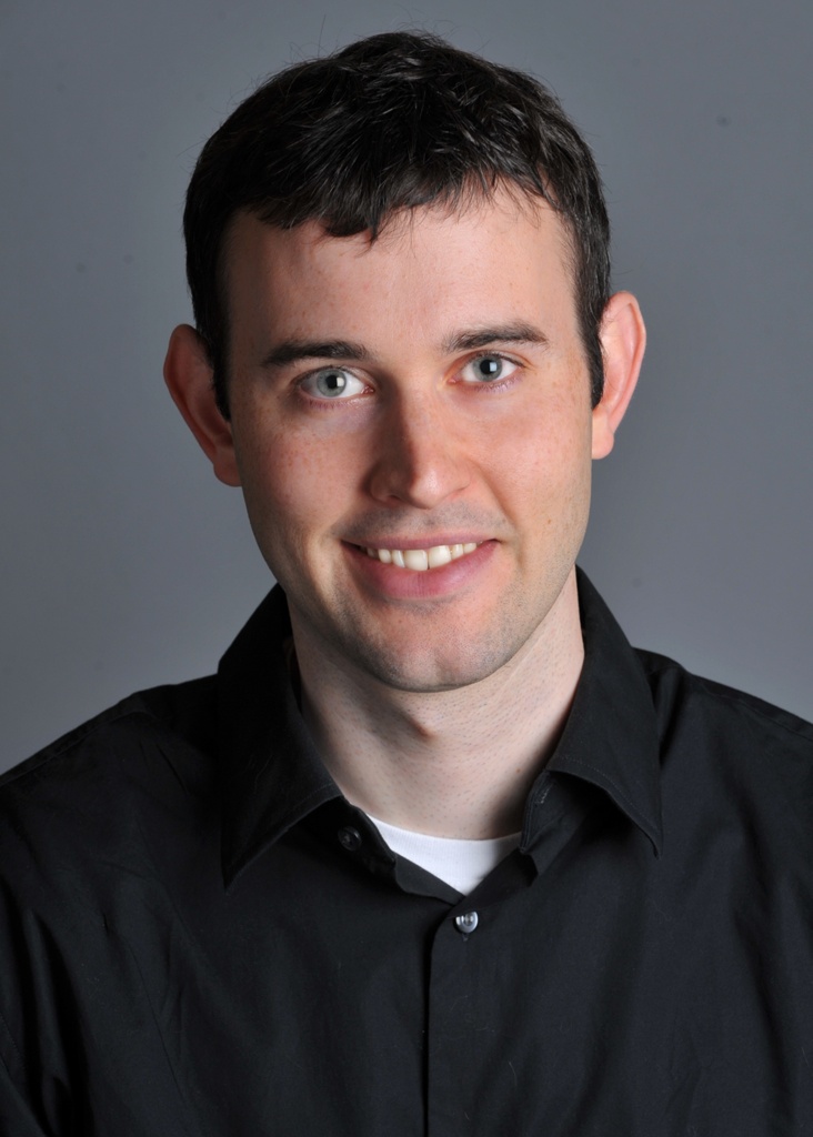
Derek (Low Frequency Image)
Nutmeg (High Frequency Image)
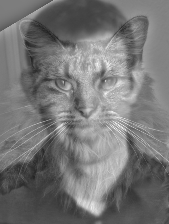
Detmeg (Low σ = 5, High σ = 23)
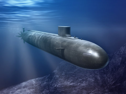
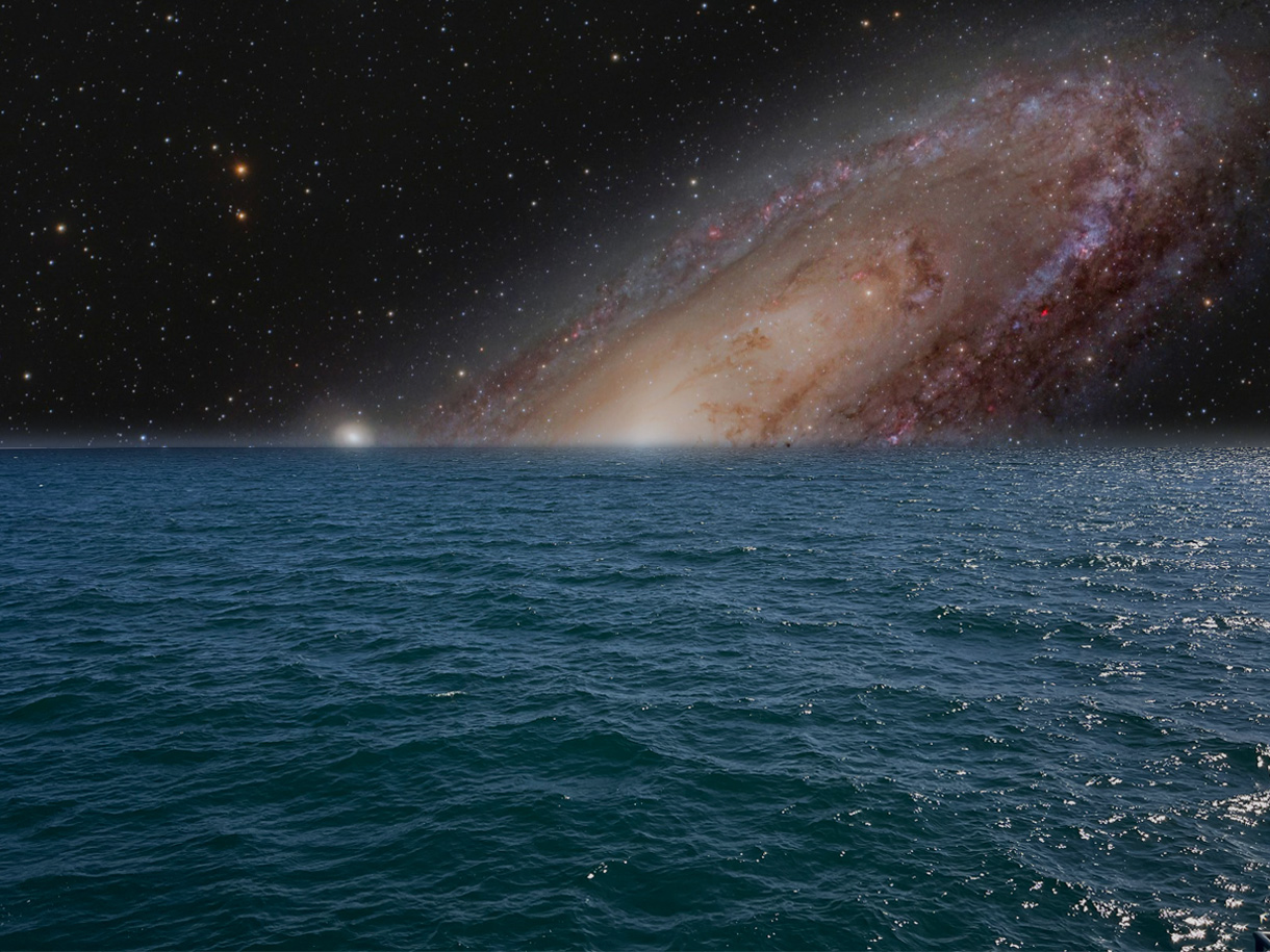
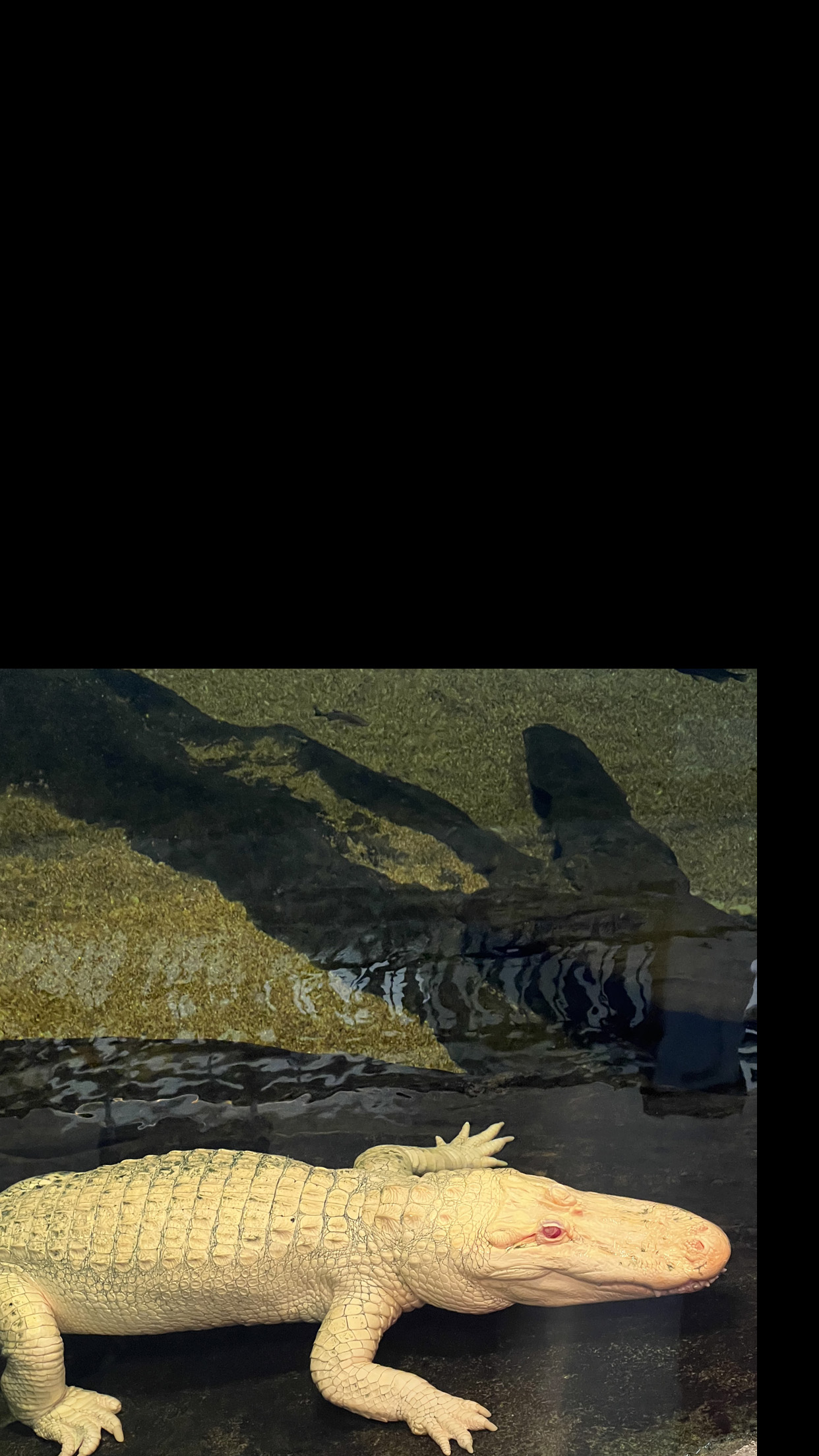
Submarine (Low Frequency Image)
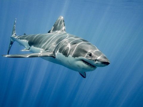
Shark (High Frequency Image)

Sharksub (Low σ = 4, High σ = 2.5)
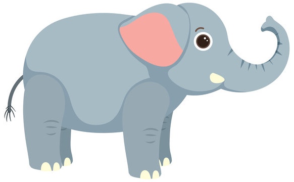
Elephant Clip Art (Low Frequency Image)
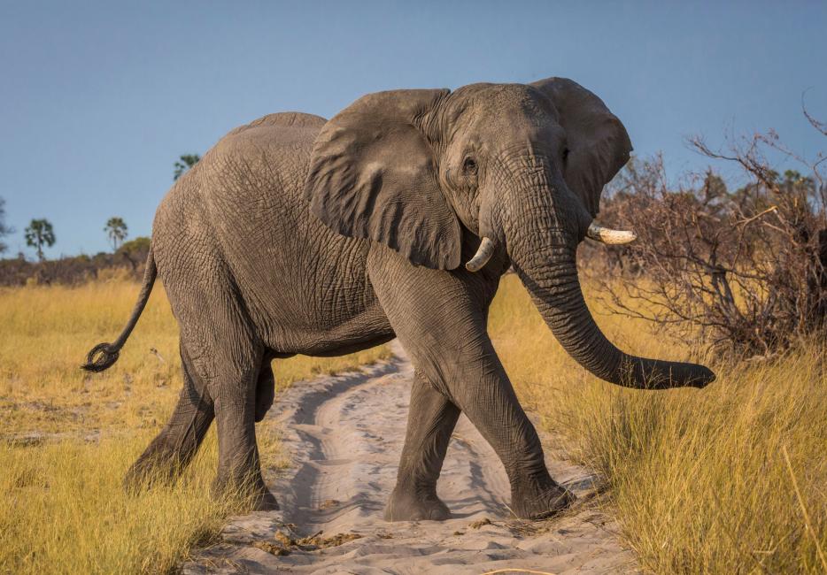
Elephant Picture (High Frequency Image)
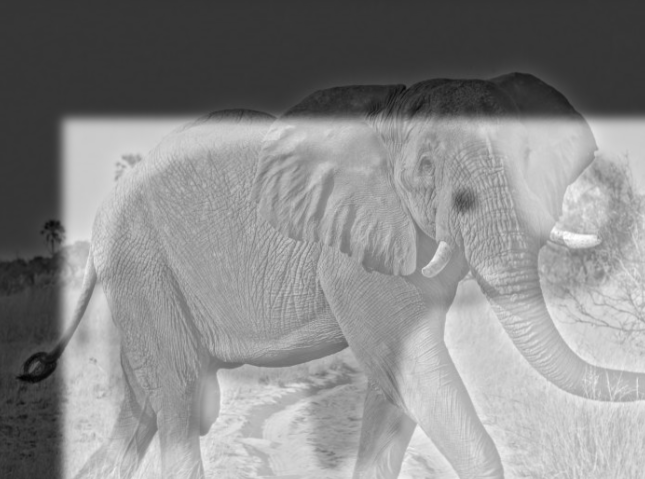
Elephants??? (Failed) (Low σ = 5, High σ = 10)
I thought it would've been cool to see a clip art from afar and a real elephant up close. It looks okay, but not as good as the Sharksub. I believe it failed because the elephants weren't in a similar orientation.
So, I realized that for a hybrid image to look great, both images need to be in a relatively similar orientation.
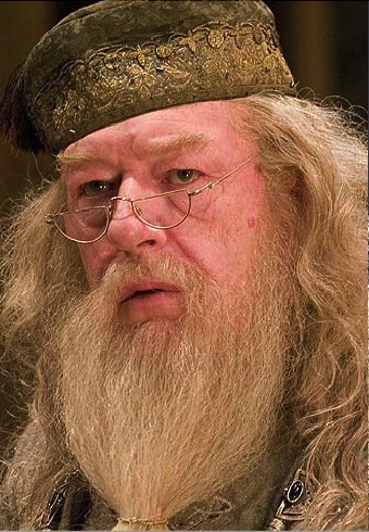
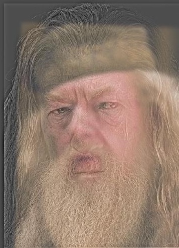
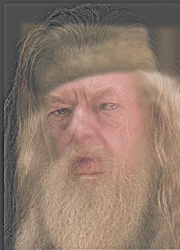
Dumbledore (Low Frequency Image)
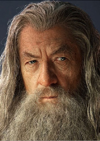
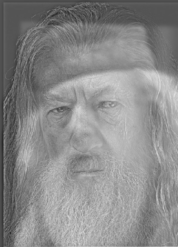
Gandalf (High Frequency Image)
Dumbledalf (Low σ = 3.5, High σ = 4)
Dumbledore

Dumbledore (Low Frequency)
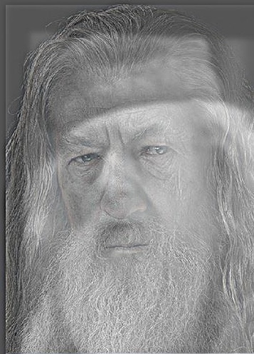
Gandalf
Gandalf (High Frequency)
Dumbledalf (Hybrid)
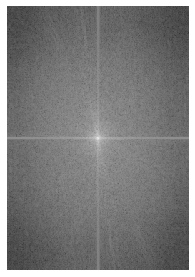
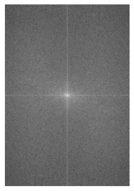
Since all signals can be decomposed into a sum of sine waves, we can map the amplitudes of each frequency. We end up getting an
amplitude spectrum. Above is the different amplitude spectrums for the Dumbledalf images.
Both Frequencies Grayscale
Only Low Frequency Colored
Only High Frequency Colored
High and Low Frequency Colored
We can add color to emphasize the high frequency, the low frequency, or both! I kept the high and low sigmas the same to see what only color does to the hybrid image. The low frequency colors
really emphasize the general color of the image, and the high frequencies give more emphasis on small details. For example, the picture with only the high frequency colored makes some of Gandalf's facial
features more noticable. However, I believe having both frequencies colored gives the best effect.
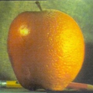
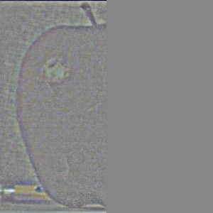
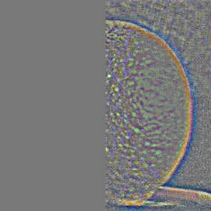
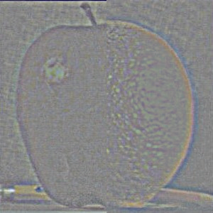
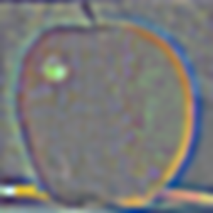
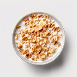
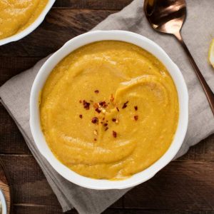
Multi-resolution Blending and the Oraple Journey
Part 2.3: Gaussian and Laplacian Stacks
In image blending using Gaussian and Laplacian stacks, we create blurred versions of the images to isolate low-frequency and high-frequency components.
A Gaussian stack consists of several levels of progressively blurred images, capturing the overall structure and low-frequency information. In contrast,
a Laplacian stack is generated by calculating the difference between consecutive levels of the Gaussian stack, which retains the high-frequency
details essential for edge detection. The blending is performed by combining these stacks with a mask that controls the contribution of each image at various levels.
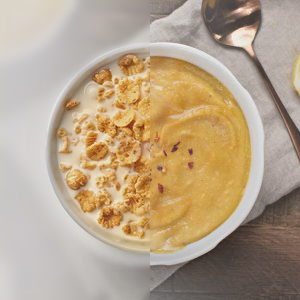
The blending equation can be expressed as:
Blended_Image(k) = Mask(k) × Image_A(k) + (1 - Mask(k)) × Image_B(k)
Here, Blended_Image(k) is formed by blending the images at each level k, using the respective mask to control
the blending amount. This method effectively merges the low-frequency components from one image with the high-frequency details
from another, resulting in a seamless transition between the two.
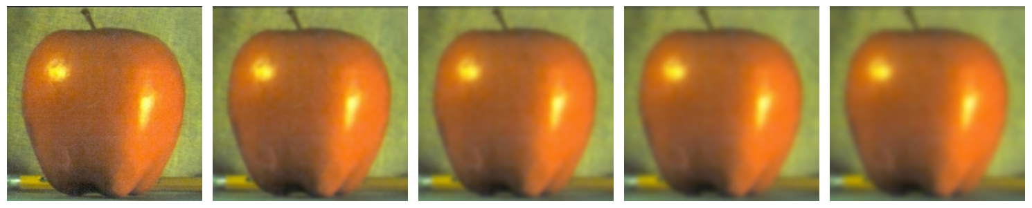
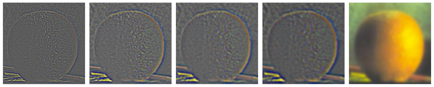
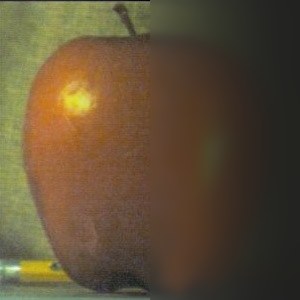
Apple Gaussian Stack
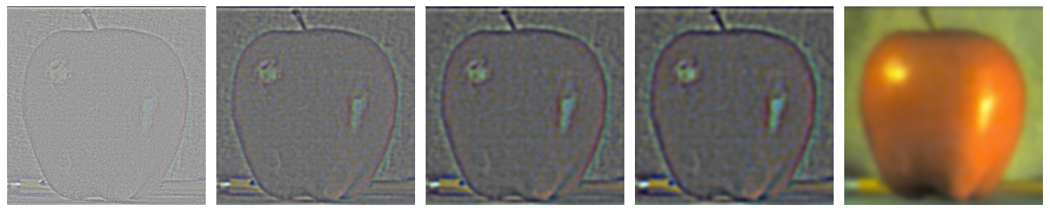
Apple Laplacian Stack
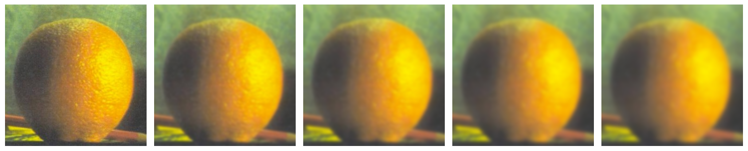
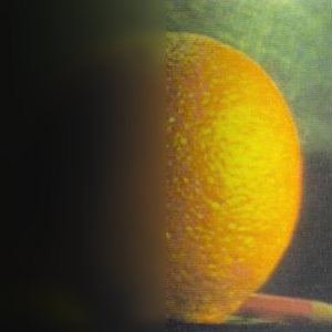
Orange Guassian Stack