Introduction
In this project, I implemented and explored NeRF. I started with implementing a neural field for a 2D image before moving on and extending the idea to a full neural radiance field.
Part 1: Fit a Neural Field to a 2D Image
Architecture
The architecture used for the 2D Neural Field was a "Multilayer Perceptron (MLP) network with Sinusoidal Positional Encoding (PE) that takes in the 2-dim pixel coordinates, and output the 3-dim pixel colors."
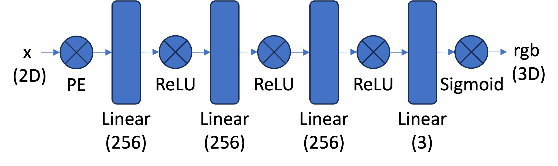
Structure of the network's architecture from the spec
Training & Sampling
The network is structured with multiple layers and utilizes activation functions such as ReLU and Sigmoid to ensure accurate color predictions. To prevent running out of memory, it trains in batches. During training, I adjusted the network's parameters such as the frequency level, channel size, learning rate, layer depth, etc to see how it affects the result.
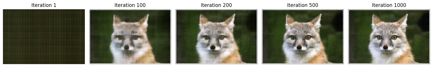
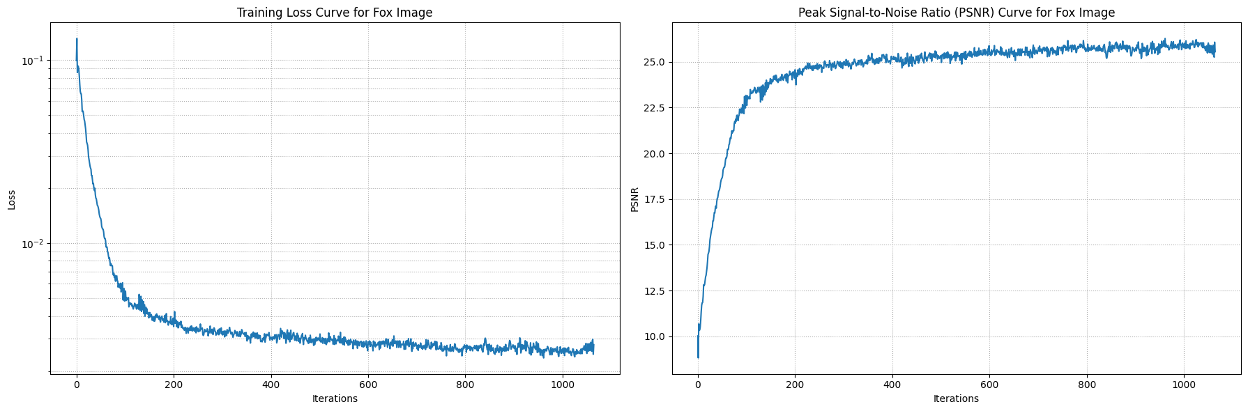
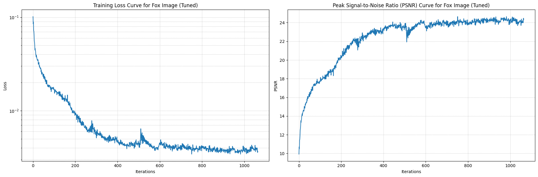
Outcomes:
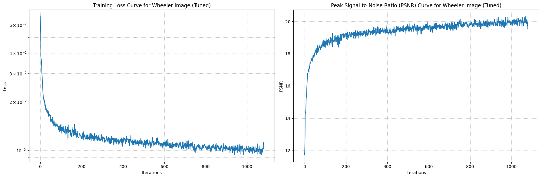
I tuned the parameters the same way for both.
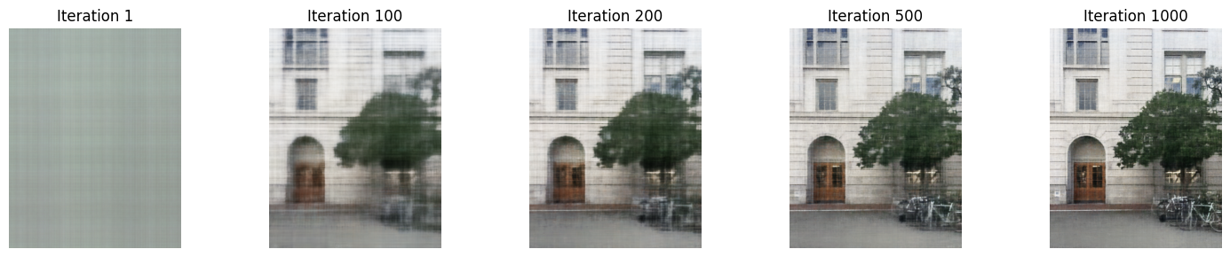
I assuming the tuned image is more "blended" due to the max frequency being lower for the positional encoding. This may have caused the
network to lose the detail positional information, which caused it to generalize the color. Also, lowering the channel size for the layers
also added to the "blended" effect because the network is capturing less information.
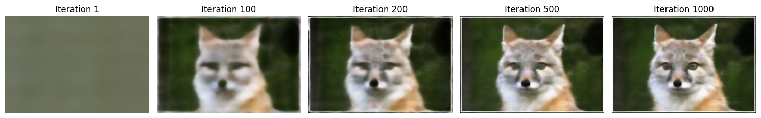
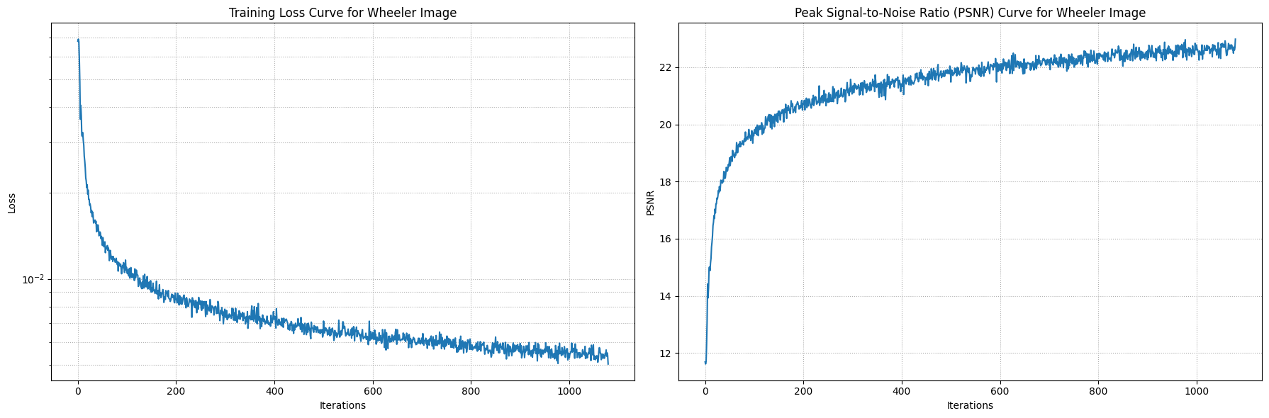
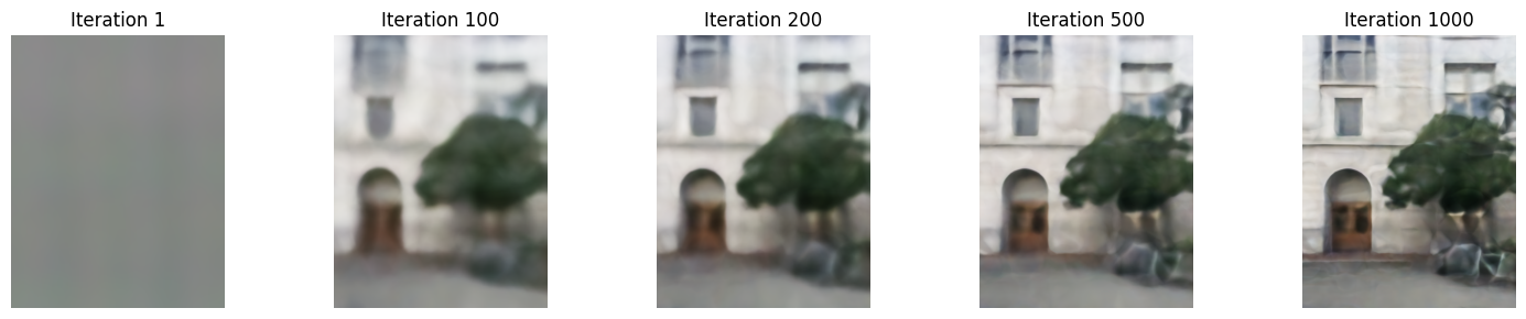
I trained both images with 1000 iterations and randomly sampled 10,000 pixels at each iteration.
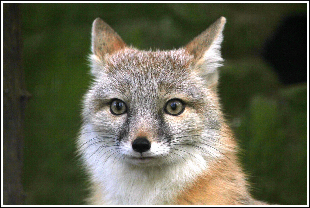
Original Fox Image
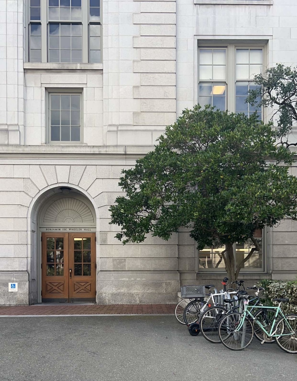
Original Wheeler Image
Part 2: Fit a Neural Radiance Field from Multi-view Images
Part 2.1: Create Rays from Cameras
In order create rays from the cameras, we implemented three functions that work together to produce the rays.
Camera to World Coordinate Conversion
This function takes a c2w matrix (or extrinsic matrix) that transofrms the camera coordinates to the world coordinates. This was matrix multiplication between c2w and x_c, the coordinate respect to camera space. I did the batched matrix multiplication using einsum, because I batched the inputs by number of images and number of pixels. Using einsum made it easier because I didn't have to worry about reshaping; the einsum notation took care of it.
Pixel to Camera Coordinate Conversion
This function takes pixel coordinates multiplies it with the intrinsic matrix to output the camera coordinate of the pixel. Similarly, I used einsum to do the
batch matrix multiplication.
Intrinsic Matrix:
f is the focal length and o is the principal point
\begin{align}
\mathbf{K} = \begin{bmatrix} f_x & 0 & o_x \\ 0 & f_y & o_y \\ 0 & 0 & 1 \end{bmatrix}
\end{align}
Pixel to Ray
This function creates the rays of each pixel in the image with respect world coordinate space. The origin ray is the location of the camera, and the direction of the ray can be found by choosing a pixel and finding its world coordinate and subtracting it from the orign ray. This computation gives the ray through that point. We used the normalized ray direction so we divided by the norm. \begin{align} \mathbf{r}_o = -\mathbf{R}_{3\times3}^{-1}\mathbf{t} \end{align} \begin{align} \mathbf{r}_d = \frac{\mathbf{X_w} - \mathbf{r}_o}{||\mathbf{X_w} - \mathbf{r}_o||_2} \end{align}
Part 2.2: Sampling
Sampling Rays from Images
We random sample rays from images. This function samples N rays, or pixels, from the image, and returns the ray origin, direction, and pixel color. This function leverages the helper functions from part 2.1. One caveat is that we need to make sure to translate the pixel grid by +0.5 to get the center of the pixel, because that is where the origin is.
Sampling Points along Rays
This function uniformly samples points along the ray. If we are training, then it introduces a slight perbutation to the points. This prevents the model from overfitting. The pebutation can't be too large otherwise the model won't learn properly.
Part 2.3: Putting the Dataloading All Together
We created a custom dataset that randomly samples pixels from the multiview images.
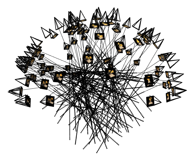
100 randomly sampled rays over the 100 training images
(1 ray per image)
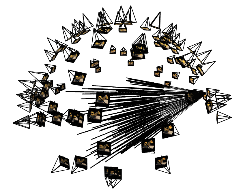
100 randomly sampled rays over one of the training images
Part 2.4: Neural Radiance Field
Architecture
To design a neural network capable of mapping 3D world coordinates and ray directions to pixel values, we need a deeper architecture. I used a predefined structure consisting of 12 linear layers, ReLU activations, and the positional encoding (PE) of the x-coordinates and ray directions which are concatenated into the middle of the MLP. The network is designed to output two results: a 1D density value and a 3D RGB vector. This means the network predicts not just the color but also the density of the 3D points
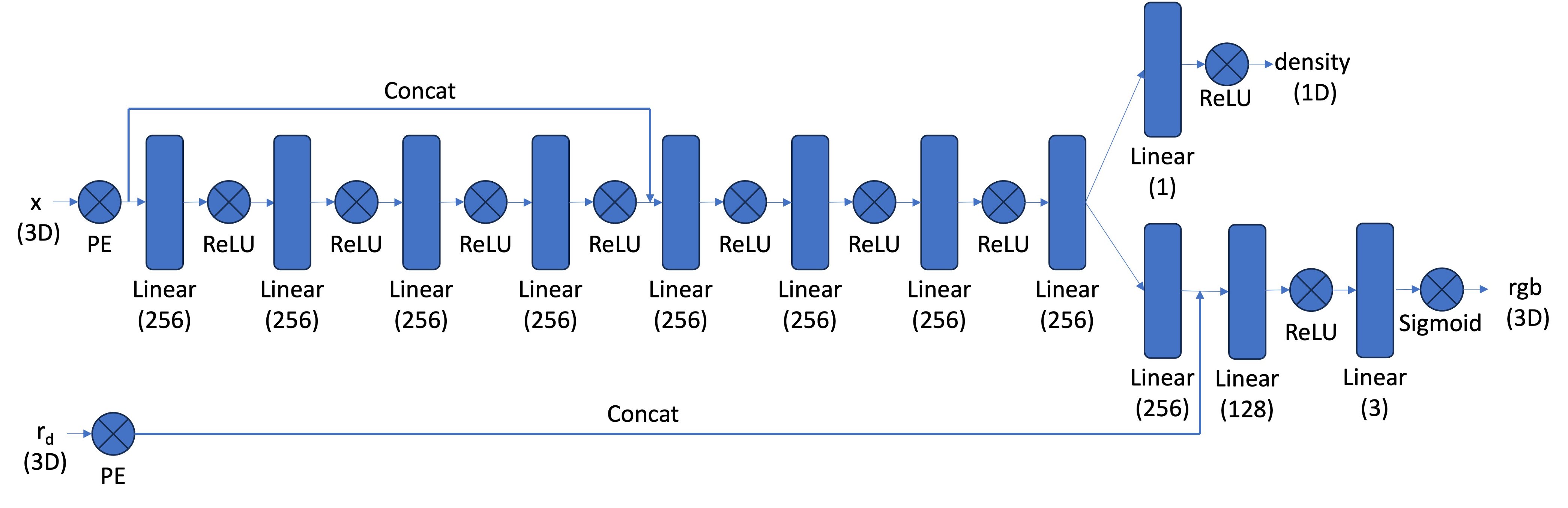
Structure of the network's architecture from the spec
Part 2.5: Volume Rendering
To get pixel color of the view, we essentially add up a weighted representation of the color of each point the model
predicted along the ray. I created a function that implemented the discrete approximation of the continuous volume rendering
function.
Continuous version of the volume rendering function:
\begin{align} C(\mathbf{r})=\int_{t_n}^{t_f} T(t) \sigma(\mathbf{r}(t))
\mathbf{c}(\mathbf{r}(t), \mathbf{d}) d t, \text { where } T(t)=\exp \left(-\int_{t_n}^t \sigma(\mathbf{r}(s)) d s\right)
\end{align}
Discrete approximation of the volume rendering function:
\begin{align}
\hat{C}(\mathbf{r})=\sum_{i=1}^N T_i\left(1-\exp \left(-\sigma_i \delta_i\right)\right) \mathbf{c}_i, \text { where } T_i=\exp
\left(-\sum_{j=1}^{i-1} \sigma_j \delta_j\right)
\end{align}
Results:
I trained over 10,000 iterations. At each iteration, I randomly sampled 50 images and 10,000 rays over the images, so 200 rays per image. I used the hyperparameters outlined in the project spec.
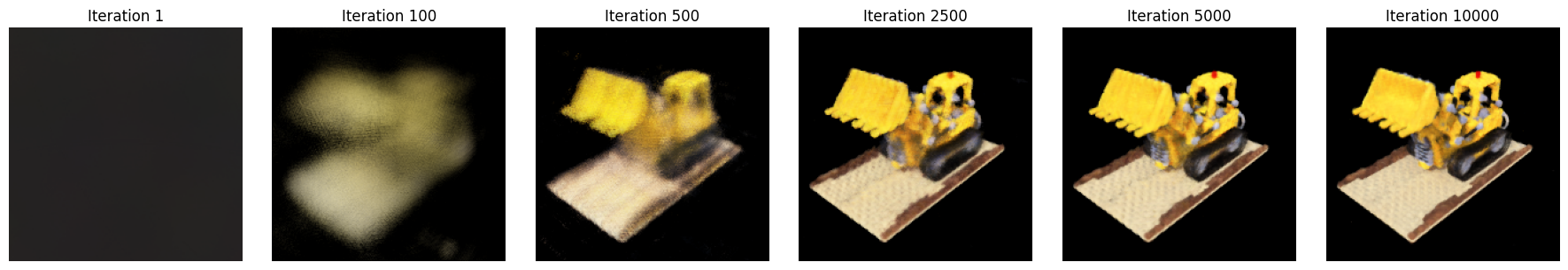
Visualization of training
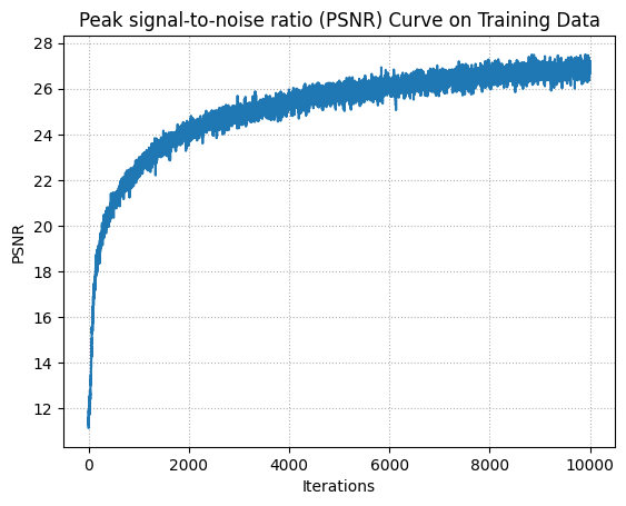
PSNR on Training Data

PSNR on Validation Data
Background Color
Render Model
Depth Map